Time-series Decomposition of Precipitation Data Using R and NASA Giovanni
This tutorial will demonstrate how to import a time series data set stored in .csv
format into R. It will explore data classes for columns in a data.frame
and will walk through how to convert a date, stored as a character string, into a date class that
R can recognize and plot efficiently.
The daily precipitation data are collected using Giovanni , a Web application developed by the GES DISC to provide a
simple, intuitive way to visualize, analyze, and access vast amounts of Earth science remote sensing data, particularly
from satellites. Giovanni includes data for aerosols, atmospheric chemistry, atmospheric temperature and moisture, and
rainfall. Giovanni also includes output from assimilation models covering a wealth of atmospheric, land surface and
oceanographic parameters. New products that superseed the TMPA datasets are now produced under the Global Precipitation
Measurement (GPM) umbrella with the Integrated Multi-satellite Retrievals for GPM (IMERG) algorithm.
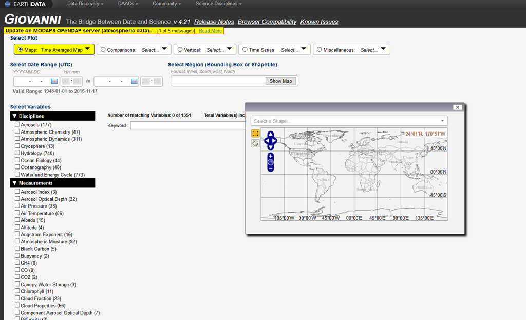
Giovanni offers a user friendly web-based environment to explore interactively various remote sensing atmospheric data. With a few mouse clicks,the user can easily obtain remote sensing or model information from around the globe, without the overhead of first having to download the data and understand complicated data formats before initiating the intended analysis. Access is provided through a common Web browser, so the user does not need special applications beyond what is available on a typical personal computer.
From a web page the user is able to select the spatial area “box” for the desired region via a Java image map applet or manually enter the coordinates defining the bounding box. The user also selects the temporal range for the data, one or more parameters from this data set, and the desired output type (ASCII or one of several plot types). For the plot selections, several color options are also available. The user is then able to refine this analysis and download the results. ASCII output is useful for GIS or other user applications, and the plots generated can be extracted into the user’s final report or paper. For more detailed analysis, links to the data are available so the user can download the entire data set for further local analysis. Depending on the choice of parameters, the majority of users will see the online results in a matter of seconds while online manipulation of larger amounts of data (either spatially or temporally) may take several minutes. Even in this more extreme case, the time from the inception of an analysis ; idea to actually seeing the results is drastically reduced and the most tedious aspects of the analysis areissues that the user bypasses in their entirety!
The purpose of the 3B42 algorithm is to produce TRMM-adjusted merged-infrared (IR) precipitation and root-mean-square (RMS) precipitation-error estimates. The algorithm consists of two separate steps. The first step uses the TRMM VIRS and TMI orbit data (TRMM products 1B01 and 2A12) and the monthly TMI/TRMM Combined Instrument (TCI) calibration parameters (from TRMM product 3B31) to produce monthly IR calibration parameters. The second step uses these derived monthly IR calibration parameters to adjust the merged-IR precipitation data, which consists of GMS, GOES-E, GOES-W, Meteosat-7, Meteosat-5, and NOAA-12 data. The final gridded, adjusted merged-IR precipitation (mm/hr) and RMS precipitation-error estimates have a daily temporal resolution and a 0.25-degree by 0.25-degree spatial resolution. Spatial coverage extends from 50 degrees south to 50 degrees north latitude.
Key Strengths:
- Uniquely offers high spatial and temporal resolution precipitation estimates over a relatively long period of record (since 1998)
- Useful for investigating the climatological distribution of rainfall, and its frequency and intensity Useful for validation of tropical precipitation in climate models, provided that care is taken to put the data on comparable grids using conservative re-gridding and to use accumulated (rather than instantaneous) precipitation
Key Limitations:
- Complex algorithms are required to translate indirect and infrequent satellite measurements into high-resolution gridded precipitation estimates at regular time intervals
- TRMM precipitation radar algorithm likely underestimates precipitation in (a) regions of intense convection over land and (b) higher latitudes
- As a Climate Data Record with global coverage, GPCP should be preferred over TRMM for large-scale climate variability studies
Due to the fact that TMPA timeseries are built up with estimates from constantly varying data sources, it is likely
that inhomegeneities in the temporal record exist. Each precipitation field should be interpreted as the best estimate of
precipitation in each grid point at the observation time. In general, as a high-resolution precipitation product,
TMPA does not have the same homogeneity goals as a climate dataset like GPCP v2.2.
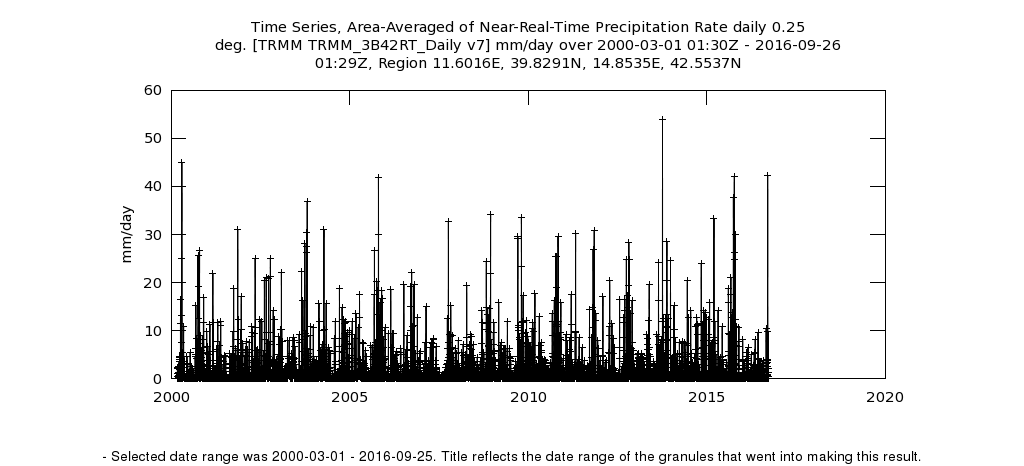
Data can be saved in several different format including graphic formats and timeseries (e.g. comma delimited format).
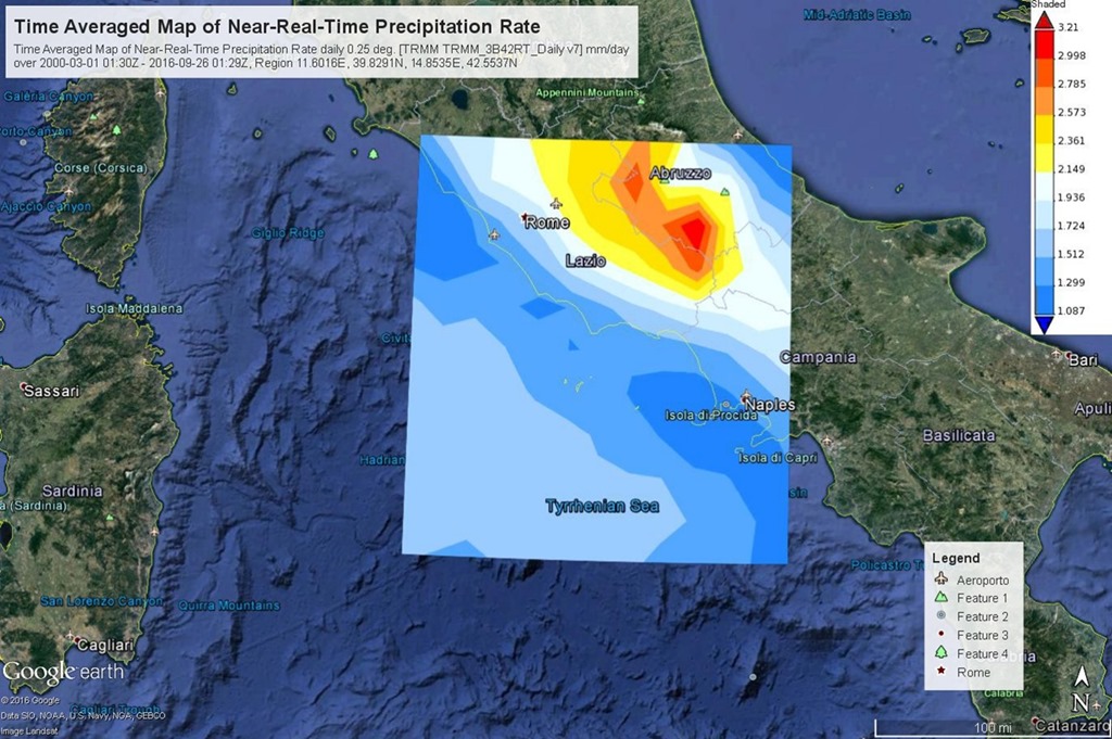
This example of the new Version 7 TMPA-RT data product shows a rainfall accumulation map in the Rome region between 2000
and 2016 generated with Giovanni.
The data that we will use is in .csv (comma-separated values) file format.
The .csv format is a plain text format, where each value in the dataset is separate by a comma and each
“row” in the dataset is separated by a line break. Plain text formats are ideal for working both across platforms
(Mac, PC, LINUX, etc) and also can be read by many different tools. The plain text format is also less likely to become
obsolete over time.
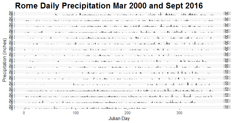
The Seasonal Trend Decomposition using Loess (STL) is an algorithm that was developed to help to divide up a time
series into three components namely: the trend, seasonality and remainder. The methodology was presented by Robert
Cleveland, William Cleveland, Jean McRae and Irma Terpenning in the Journal of Official Statistics in 1990.
The STL is available within R via the stl function.
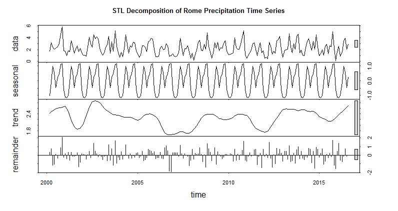
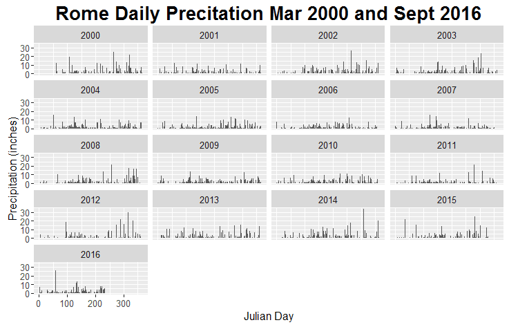
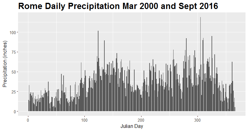
The four graphs are the original data, seasonal component, trend component and the remainder and this shows the periodic seasonal pattern extracted out from the original data. There is a bar at the right hand side of each graph to allow a relative comparison of the magnitudes of each component. For this data the change in trend is less than the variation doing to the monthly variation.
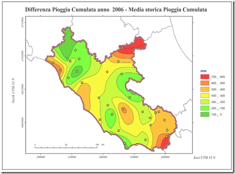
The trend component shows a marked insufficiency of precipitation in 2006, confirmed also by the two lines below zero
in the remainder component. this is confirmed by the historical report of the Roman authorities:
The year 2006 was characterized by a general lack of liquidity and snowfall and temperatures significantly above the
average of the entire national territory. Such lack of precipitation has also been reflected in Lazio, causing abnormal
weather-hydrological situations, in particular with reference to the period September - December 2006.
The smallness of the snow cover at the end of this year on the Apennines, and the data available from the monitoring of
the most sensitive sources to annual variations in precipitation, in the case of persistence of water supply deficit,
inducing to expect for the coming months outflows reduced , with possible critical as regards both the irrigation
requirement that it caters for the surface water resource, both for the respect of the conditions of outflow
minimum
subsistence of the waterways.
There were no critical situations regarding the drinking water supply.
After over 17 years of productive data gathering, the instruments on TRMM were turned off on April 8, 2015. The spacecraft re-entered the Earth’s atmosphere on June 15, 2015, at 11:55 p.m. EDT, over the South Indian Ocean, The multi-satellite 3B42*/TMPA product will continue to be produced through early 2018 when the transition from 3B42* to IMERG will be complete.