Predicting the presence of Fall Armyworm with Machine Learning
In December 2019, FAO launched the pioneering Global Action for Fall Armyworm Control as an urgent
response to the rapid spread of FAW. The three-year global initiative takes radical, direct,
and coordinated measures to strengthen prevention and sustainable pest control capacities at a global level.
It complements and bolsters ongoing FAO activities on FAW.
The Global Action has established a global coordination mechanism for an open and collaborative dialogue
towards science-based solutions. It has also supported the establishment of National Task Forces on FAW,
and the mobilization of resources for applied research geared towards practical and efficient solutions.
The FAW Monitoring and Early Warning System (FAMEWS) is a free mobile application for Android cell phones
from the Food and Agriculture Organization of the United Nations (FAO) for the real-time global monitoring
of the Fall Armyworm (FAW).
This multi-lingual tool allows farmers, communities, extension agents and others
to record standardized field data whenever they scout a field or check pheromone traps for FAW.
Data from the app provides valuable insights on how FAW changes over time with ecology, to improve knowledge
of its behaviour and guide best management practices.
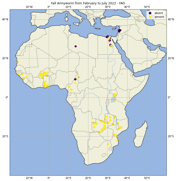
All collected data are used by FAO, countries, and partners to map and monitor current infestations. The app is designed to expand with the evolving needs of farmers, analysts, and decision-makers. The data collected by FAO through mobile applications allow you to have an idea of possible outbreaks due to agricultural pests. The data are freely provided to anyone who has an interest in analyzing them via API as detailed in the Hand-In-Hand Geospatial Platform https://data.apps.fao.org/ The data shared on the internet are very limited and report only the controlled plants, those found infected with FAW and the percentage of infection as derived data. Also, the spatial distribution of the data is very sparse and highly unbalanced and while there are many records of visits to the field where the plague has been detected there are only very few where the opposite occurs.
.png)
Adding meteorological and biophysical data to scoutings from the field
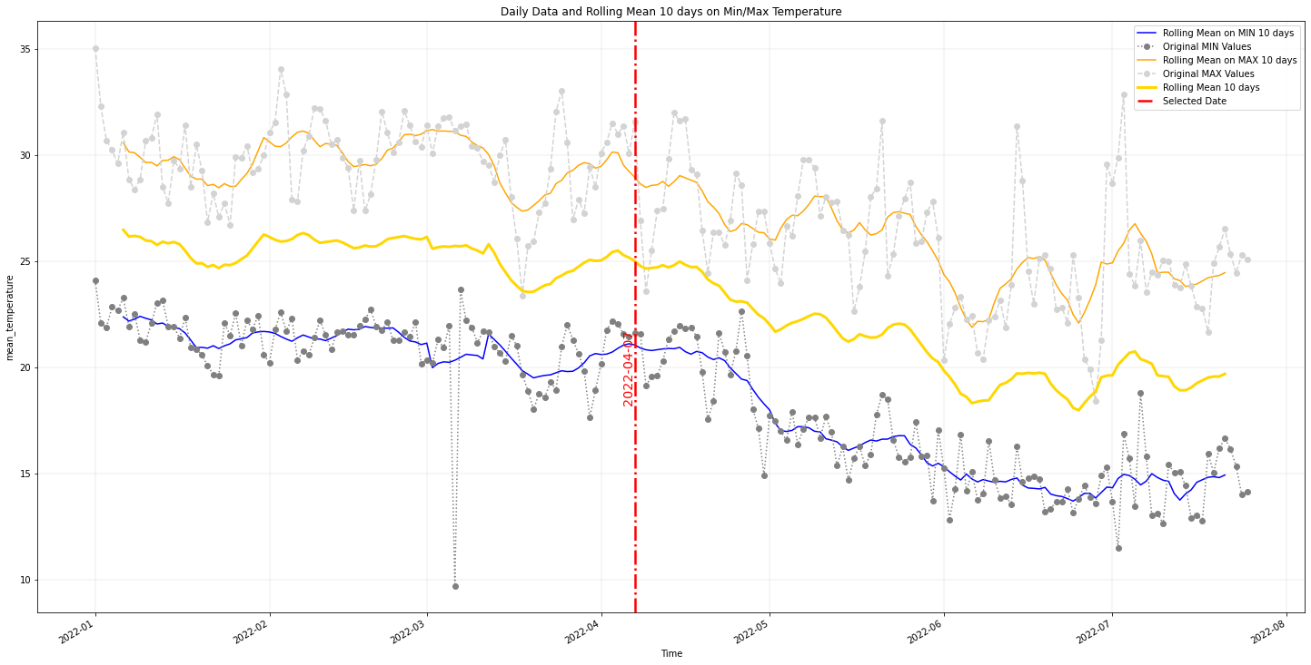
Every point collected in the field has been enriched, using latitude and longitude, with data coming from meteorological models, soil moisture and vegetation data. The data are in parts downloaded from the internet and analyzed locally and some are gathered from Google Earth Engine.At the end of this process evey point will have 10 days of observations associated with it. For example for the temperature the timeseries will look similar to the following image
CHIRPS Data Rainfall Estimates from Rain Gauge and Satellite Observations
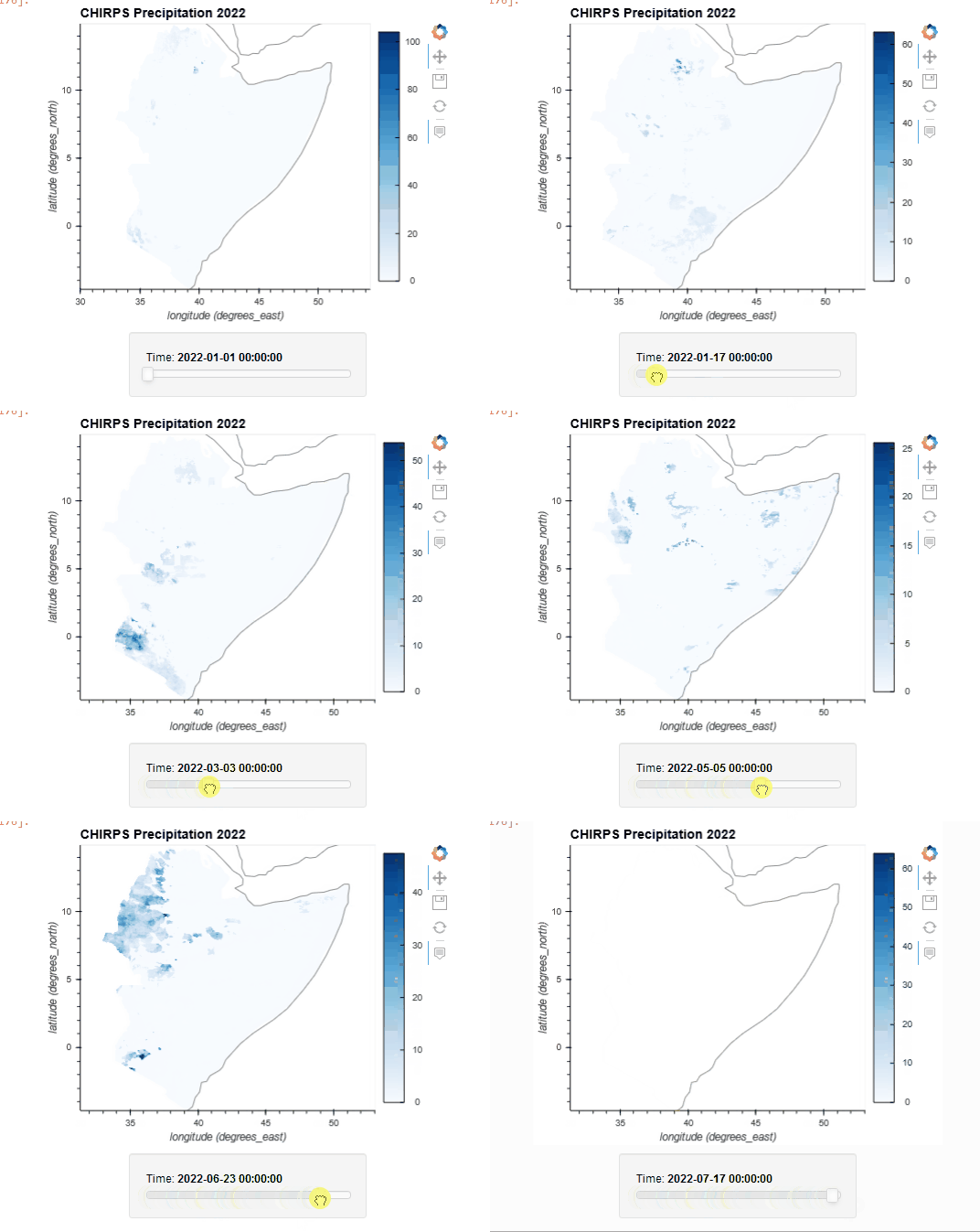
Since 1999, USGS and CHC scientists—supported by funding from USAID, NASA, and NOAA—have developed techniques for producing rainfall maps, especially in areas where surface data is sparse. Estimating rainfall variations in space and time is a key aspect of drought early warning and environmental monitoring. An evolving drier-than-normal season must be placed in a historical context so that the severity of rainfall deficits can be quickly evaluated. However, estimates derived from satellite data provide areal averages that suffer from biases due to complex terrain, which often underestimate the intensity of extreme precipitation events. Conversely, precipitation grids produced from station data suffer in more rural regions where there are less rain-gauge stations. CHIRPS was created in collaboration with scientists at the USGS Earth Resources Observation and Science (EROS) Center in order to deliver complete, reliable, up-to-date data sets for a number of early warning objectives, like trend analysis and seasonal drought monitoring.
Global Unified Temperature 0.5x0.5 Global Daily Gridded Temperature
The NOAA Physical Sciences Laboratory (PSL) conducts weather, climate and hydrologic research to advance the prediction of water availability1 and extremes. The NOAA Global Surface Temperature Dataset (NOAAGlobalTemp) is a merged land-ocean surface temperature analysis (formerly known as MLOST). It is a spatially gridded (5° - 5°) global surface temperature dataset, with monthly resolution from January 1880 to present. We combine a global sea surface (water) temperature (SST) dataset with a global land surface air temperature dataset into this merged dataset of both the Earth's land and ocean surface temperatures. The SST dataset is the Extended Reconstructed Sea Surface Temperature (ERSST) version 5.0. The land surface air temperature dataset is similar to ERSST but uses data from the Global Historical Climatology Network Monthly (GHCN-M) database, version 4. We provide the NOAAGlobalTemp dataset as temperature anomalies, relative to a 1971-2000 monthly climatology, following the World Meteorological Organization convention. This is the dataset NOAA uses for global temperature monitoring.
Soil Moisture from GLDAS-2.1: Global Land Data Assimilation System
Global Land Data Assimilation System (GLDAS) ingests satellite and ground-based observational data products. Using advanced land surface modeling and data assimilation techniques, it generates optimal fields of land surface states and fluxes. GLDAS-2.1 is one of two components of the GLDAS Version 2 (GLDAS-2) dataset, the second being GLDAS-2.0. GLDAS-2.1 is analogous to GLDAS-1 product stream, with upgraded models forced by a combination of GDAS, disaggregated GPCP, and AGRMET radiation data sets. The GLDAS-2.1 simulation started on January 1, 2000 using the conditions from the GLDAS-2.0 simulation. his simulation was forced with National Oceanic and Atmospheric Administration (NOAA)/Global Data Assimilation System (GDAS) atmospheric analysis fields (Derber et al., 1991), the disaggregated Global Precipitation Climatology Project (GPCP) precipitation fields (Adler et al., 2003), and the Air Force Weather Agency's AGRicultural METeorological modeling system (AGRMET) radiation fields which became available for March 1, 2001 onwards. The band used is the RootMoist_inst kg/m^2 2* 949.6* Root zone soil moisture
Fraction of green Vegetation Cover
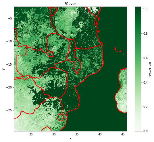
The Fraction of Vegetation Cover (FCover) corresponds to the fraction of ground covered by green vegetation. Practically, it quantifies the spatial extent of the vegetation. Because it is independent from the illumination direction and it is sensitive to the vegetation amount, FCover is a very good candidate for the replacement of classical vegetation indices for the monitoring of ecosystems.
Exploratory Data Analysis

The final dataset after the enrichment contains (image above) all the meteorological and
vegetation data gathered plus the label, presence absence of the pest, to be used for supervised classification.
Given the complexity of the data enrichment phase, it is worth spending some time to verify the
correctness of the added data, the relationship between the various components and the relationships
between the presence of the plague with weather and vegetation data.
The first issue, as we have seen, is that the data collected in the field are strongly unbalanced
by the almost exclusive presence of data with the presence of the infesting plague. Imbalanced
data typically refers to a problem with classification problems where the classes are not represented equally.
The presence/absence 2-class (binary) classification has 4810 instances (rows) and a total of 4410 instances labeled
with "present" and the remaining 400 instances are labeled with "absence".
This is an imbalanced dataset and the ratio of "presence" to "absence" instances is 4410:400 or more concisely 11:1.
The learning phase and the subsequent prediction of machine learning algorithms can be affected by
the problem of imbalanced data set. The balancing issue corresponds to the difference of the number of
samples in the different classes.
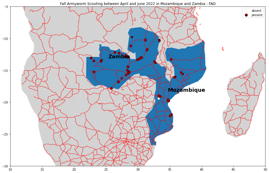
The spatial distribution of the data is also very problematic because it covers a very small area of the African continent and also at the national level the data are very scattered and in a very small number compared to the vastness of the territory. Another element that seems to influence very negatively the validity of the data collected in the field is given by the collection of field data only and exclusively along the roads and not in the innermost rural areas. Often the data collected are located in urban areas where the presence of agricultural fields should be scarce or non-existent.
According to CABI:
A threshold temperature of 10.9°C and 559 day-degrees C is required for development. Sandy-clay or clay-sand soils are suitable for pupation and adult emergence. Emergence in sandy-clay and clay-sand soils was directly proportional to temperature and inversely proportional to humidity. Above 30°C the wings of adults tend to be deformed. Pupae require a threshold temperature of 14.6°C and 138 day-degrees C to complete their development (Ramirez-Garcia et al., 1987). S. frugiperda is a tropical species adapted to the warmer parts of the New World; the optimum temperature for larval development is reported to be 28°C, but it is lower for both oviposition and pupation. In the tropics, breeding can be continuous with four to six generations per year, but in northern regions only one or two generations develop; at lower temperatures, activity and development cease, and when freezing occurs all stages are usually killed. In the USA, S. frugiperda usually overwinters only in southern Texas and Florida. In mild winters, pupae survive in more northerly locations.
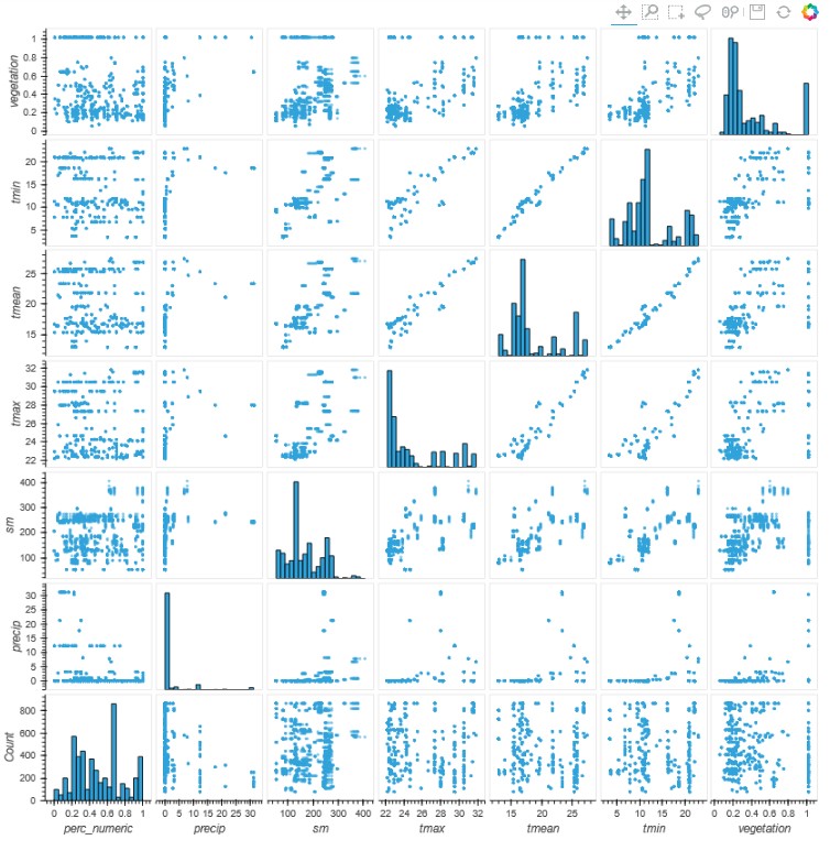
This is confirmed by the analysis of the data, the level of infestation on the fields visited by the workers shows a very poor correlation with all the parameters taken into consideration, temperature, soil moisture, vegetation and precipitation or in other words the conditions favorable to the spread of the plague are present in a large part of the African continent.
Feature Engineering
- Feature Engineering Techniques Applied
- Feature Scaling
- Under-sampling Data
Feature Scaling is a technique to standardize the independent features present in the data in a fixed range. It is performed during the data pre-processing to handle highly varying magnitudes or values or units. If feature scaling is not done, then a machine learning algorithm tends to weigh greater values, higher and consider smaller values as the lower values, regardless of the unit of the values. If we passed the data as they are to an algorithm is not using the feature scaling method then it can consider the value 350 degrees Kelvin to be greater than millimetres of rain but that’s actually not true and in this case, the algorithm will give wrong predictions. So, we use Feature Scaling to bring all values to the same magnitudes and thus, tackle this issue.
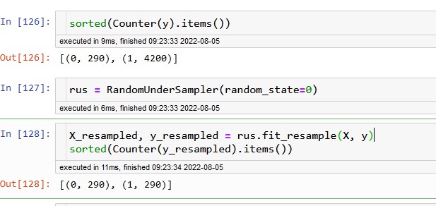
In order to have more balanced data some instances are delete from the over-represented class,
called under-sampling using the python library named Imbalanced-Learn. Imbalanced-Learn is a Python module
that helps in balancing the datasets which are highly skewed or biased towards some classes.
Thus, it helps in resampling the classes which are otherwise oversampled or undesampled.
If there is a greater imbalance ratio, the output is biased to the class which has a higher number
of examples.
The resampling of data is done in 2 parts:
Estimator: It implements a fit method which is derived from scikit-learn. The data and targets are both in the form of a 2D array
Resampler: The fit_resample method resample the data and targets into a dictionary with a key-value pair of data_resampled and targets_resampled.
The Imbalanced Learn module has different algorithms for oversampling and undersampling the Random Under Sampler has been used in this case which involves sampling any random class with or without any replacement.
Syntax:
from imblearn.under_sampling import RandomUnderSamplerParameters(optional): sampling_strategy=’auto’, return_indices=False, random_state=None, replacement=False, ratio=None
Implementation:
X_under, y_under = undersample.fit_resample(X, y)
Return Type: a matrix with the shape of n_samples*n_features
Logistic Regression - Accuracy 79%
In regression analysis, logistic regression (or logit regression) is estimating the parameters of a logistic model (the coefficients in the linear combination). It estimates the probability of an event occurring, presence absence in this case, based on a given dataset of independent variables. Since the outcome is a probability, the dependent variable is bounded between 0 and 1.
| precision | recall | f1-score | support | |
|---|---|---|---|---|
| absent | 0.88 | 0.65 | 0.75 | 57 |
| present | 0.73 | 0.92 | 0.81 | 59 |
| accuracy | 0.78 | 116 | ||
| macro avg | 0.81 | 0.78 | 0.78 | 116 |
| weighted avg | 0.80 | 0.78 | 0.78 | 116 |
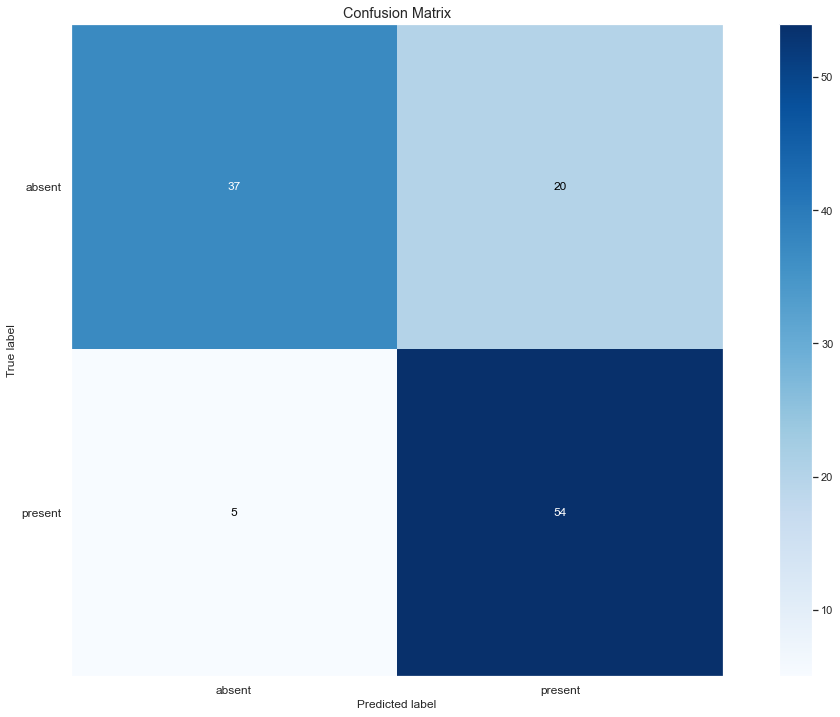
Out of 116 cases the model was able to correctly identify 37 True Positives and 54 False Positives, only 5 cases were improperly
classified as cases where mistakenly labelled as absent Fall Armyworm, while a greater number of errors is found in the erroneous
assignment of absence where there is the presence of plague.
A greater balance between the two types of errors can be achieved by slightly modifying the 50% threshold
used by default in the development of the model.
Conclusions
The model developed manages to reach an accuracy of around eighty percent, which seems good considering that
to minimize the impact of the imbalance of the collected data a large part of the data has been discarded.
In addition to having a good ability to predict the presence of FAW in eighty cases out of a hundred, it also
has a remarkable homogeneity as regards precision and sensitivity (recall) with values that are also close to
eighty percent as well.
Precision attempts to answer the question “What proportion of positive identifications was actually correct?”,
while Recall attempts to answer the question “What proportion of actual positives was identified correctly?”.
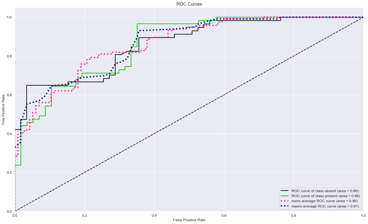
Below the ROC chart showing the performance of the classification model at all classification thresholds.
